A color Doppler image can show a sudden change in hue across a fast-flowing region, while a spectral trace can appear to hit its edge and reappear on the opposite side. This wraparound pattern is called aliasing. It arises because pulsed Doppler samples echoes at discrete intervals, so a sufficiently rapid frequency shift cannot be represented uniquely. The display has reached a sampling limit; the colors alone do not prove that the blood suddenly changed direction. [1]
Motion becomes a frequency shift
Ultrasound echoes from moving red blood cells return with a frequency slightly different from the transmitted sound. For a pulse reflected by moving scatterers, the shift depends on the blood speed, the transmitted frequency, the speed of sound in tissue, and the angle between the sound beam and motion. In simplified form, Δf = 2 f₀ v cos(θ) / c. The factor of two comes from the outward and return paths. [2]
This is a projection measurement. Motion along the beam contributes strongly; motion across it contributes less, and a perpendicular beam produces little Doppler shift. The scanner uses this frequency information to estimate direction and velocity under its assumptions.
A pulse train is also a sampling clock
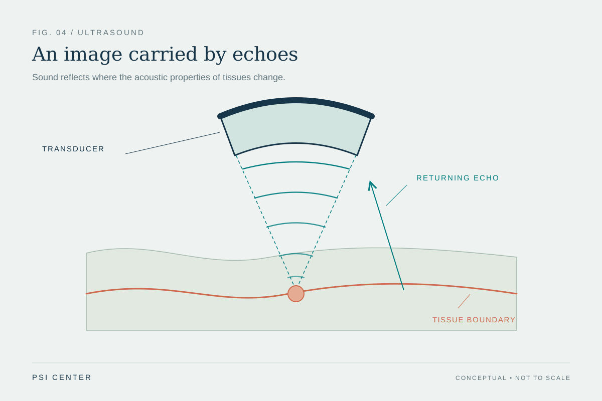
In pulsed-wave Doppler, the probe sends a short burst, listens for echoes, and repeats. Because the instrument knows when each burst was sent, it can associate returning information with a chosen depth range. The number of bursts sent per second is the pulse repetition frequency (PRF). Each echo therefore provides a sample of the changing Doppler signal, rather than a continuous record. [1]
For a repeating signal sampled at rate PRF, the Nyquist limit is half that rate: the highest unambiguous frequency shift is PRF/2. Above it, different underlying shifts can produce the same sequence of samples. The reconstructed signal folds into the display’s available range, like a wheel that seems to turn backward in a film when its spokes are sampled too slowly.
A worked example of the limit
Suppose a pulsed Doppler system samples at 4,000 pulses per second. Its simple Nyquist ceiling is 2,000 Hz. A 1,500 Hz shift fits below that ceiling, but a 2,500 Hz shift exceeds it and cannot be represented as a unique 2,500 Hz value from those samples alone. The display may wrap the excess back across its scale. This arithmetic illustrates sampling; it is not a recommended scanner setting. [1]
The wrap is not a literal reflection of the flow in space. It is ambiguity in the sampled signal. Spectral Doppler often shows a clipped peak continuing from the opposite edge; color Doppler may show an abrupt change in the color scale. The pattern warns that the displayed scale is insufficient to portray that shift unambiguously, while other image features and context still matter.
Depth competes with sampling speed
A pulse must travel to a reflector and back before the system can safely send another pulse for the same line. Deeper targets take longer round trips, which constrains how quickly they can be sampled. The review of vascular-access Doppler describes this inverse relationship between sample depth and PRF: as depth increases, the available sampling rate and therefore the unambiguous shift limit can fall. [1]
This is a design tradeoff built into pulse-echo measurement. Pulsed Doppler provides depth selection, but the time needed to listen for deep echoes limits the sampling clock. Continuous-wave Doppler avoids the same pulsed sampling ceiling for high shifts, but it does not isolate a single depth along the beam. No mode removes every limitation; each answers a different measurement question. [2]
Changing the display does not add missing information
A display scale can be shifted so that more of the range appears on one side of zero, which may help show a directional waveform. But shifting the baseline only rearranges the available display; it does not increase the underlying sampling rate. A higher PRF can raise the Nyquist limit, although depth and system timing constrain how far it can be raised. Changing the transmitted frequency or beam angle also changes the Doppler shift itself, so those changes affect the measurement conditions rather than simply making the original signal clearer. [1]
The practical lesson is to read the signal as a measurement with boundaries. Aliasing can flag that the observed shift exceeds the unambiguous range, but a color transition is not by itself a diagnosis or a reliable velocity estimate. The method, sample location, angle, and other sources of error affect interpretation. These principles explain an imaging artifact; they do not prescribe settings for a particular examination.
Explore the physics: an explanatory diagram
Sources & further reading
- Basics for performing a high-quality color Doppler sonography of the vascular access Journal of Ultrasound (2021)
- Essential notes on the physics of Doppler ultrasound BJA Education (2020)
Sources checked: 5 November 2026. The calculations illustrate physical models; they are not clinical settings.
Prepared for the independent PSI Center reading library. About edition dates and source checking.
This explainer describes scientific principles. It does not assess individual treatment choices.