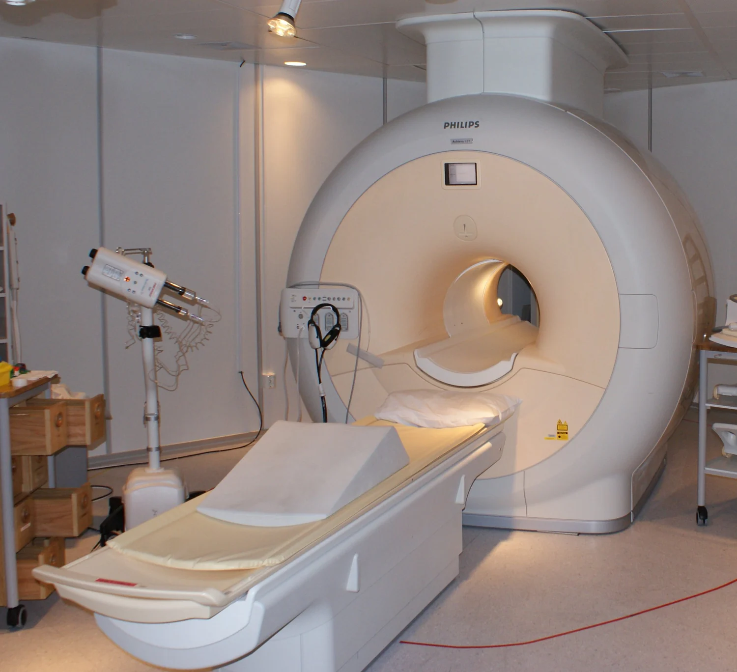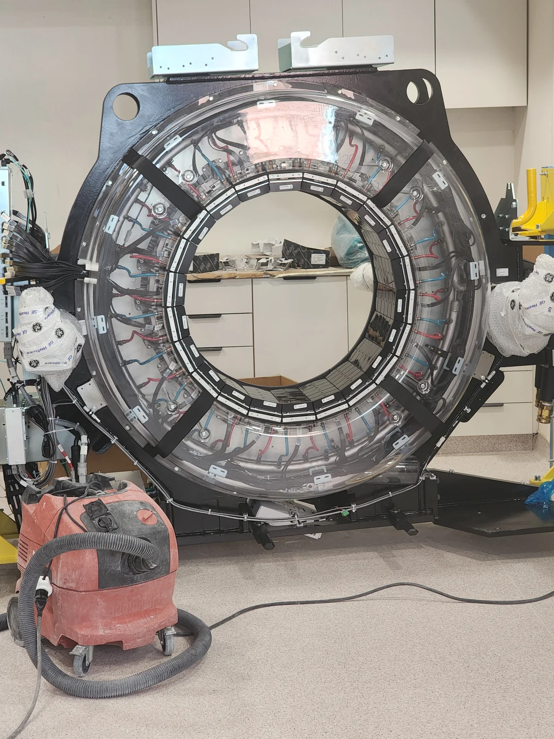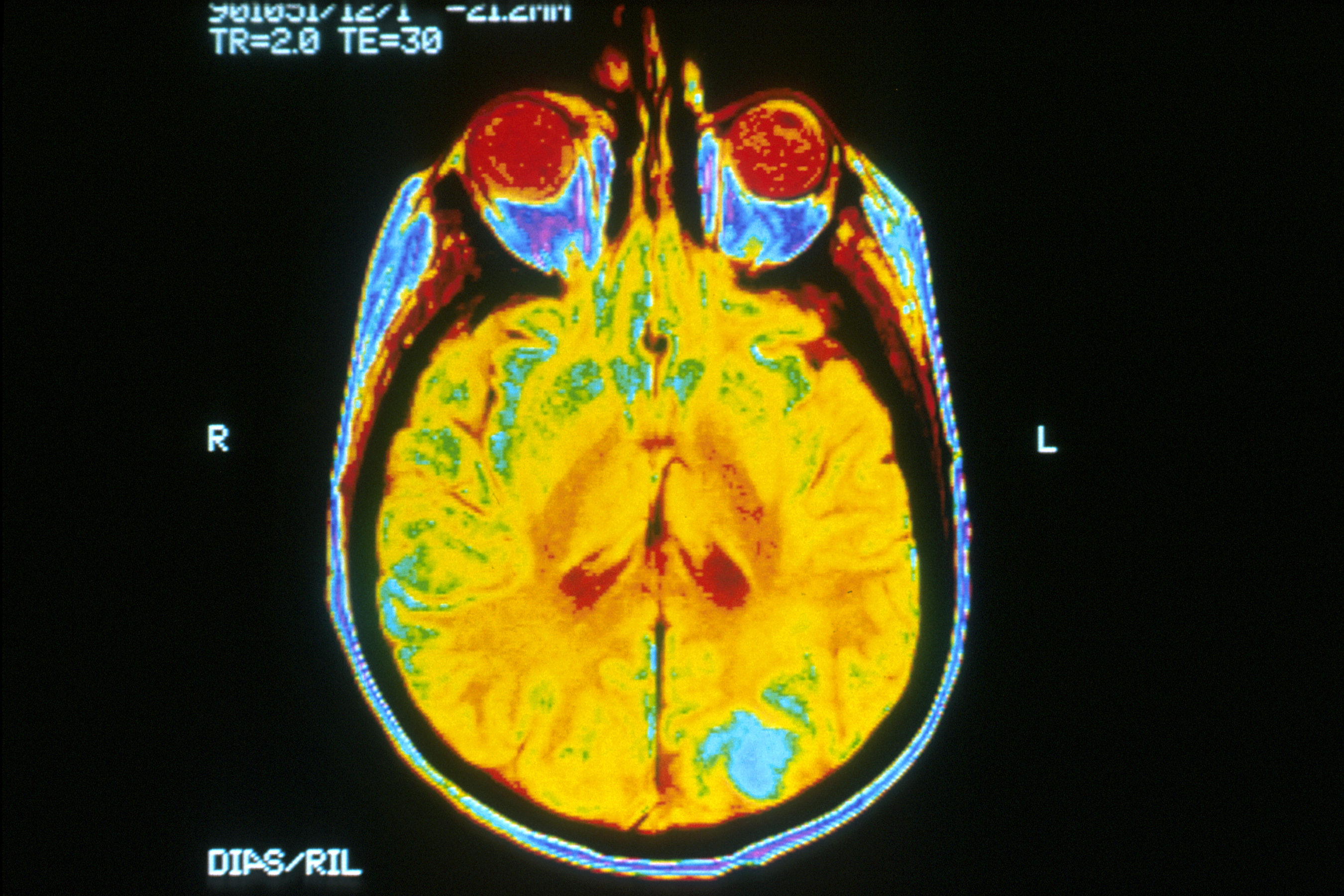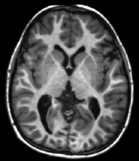
An MRI scanner with many receiver channels can collect signals from several coil elements at once. The important advantage is not simply that it has more “ears.” Each element hears the body differently, and those spatial differences can help the reconstruction distinguish locations that would otherwise overlap when fewer measurements are taken. That can shorten acquisition, but it also makes image quality depend on the array’s geometry and the noise in each channel. [1]
A receiver coil has a spatial fingerprint
MRI gradients encode position by changing the phase and frequency of the returning signal. A receive coil adds another kind of information: its sensitivity varies across space. A small element close to one region may detect that region strongly and a distant region weakly. The resulting pattern is not a sharp boundary or a pixel map; it is a smoothly varying sensitivity profile that overlaps with the profiles of other elements.
An array combines these overlapping views. The signal from one location may be weak in one channel and stronger in another, while a different location has a different pattern across the same channels. Reconstruction can use those differences as additional spatial clues. The coil therefore participates in encoding, even though the gradients and radiofrequency excitation still do important parts of the measurement. [1]
How different coil views replace some measurements
A conventional Fourier MRI acquisition samples a planned set of points in k-space, the space of spatial frequencies used to form the image. Parallel imaging deliberately collects fewer phase-encoding steps than a fully sampled acquisition. If the missing measurements were simply ignored, the image would contain overlapping copies, or aliasing. Sensitivity encoding (SENSE) instead treats each coil channel as a different weighted view of those overlaps and solves for the underlying image using both the measured data and the coil sensitivity patterns. [1]
This is a reconstruction problem, not a camera trick that creates new photons or restores every omitted detail. It works when the coil profiles provide enough independent information to separate the overlapped locations and when calibration describes those profiles well enough. The first SENSE report demonstrated the idea in phantom and in-vivo imaging, including a two-coil brain acquisition at half the conventional scan time and five-coil cardiac images at one-third of conventional time. Those are demonstrations in the study’s configurations, not guaranteed reductions for any scan. [1]
Acceleration trades sampling for noise
Fewer acquired phase-encoding steps can reduce scan time, but the reconstructed image generally pays a signal-to-noise penalty. Coil geometry adds another factor. If two locations produce very similar patterns across the available elements, the reconstruction has trouble telling them apart; solving that ambiguity amplifies noise. MRI physicists describe this spatially varying noise penalty with the geometry factor, or g-factor. A favorable array has profiles that are sufficiently distinct in the direction being accelerated.
Adding elements can improve those distinctions, but channel count alone does not set performance. Element placement, size, overlap, coupling, electronics, field strength, anatomy, and the chosen acceleration direction all matter. Calibration errors or motion between calibration and image acquisition can also undermine the assumed sensitivity maps. The same array can perform differently for different image regions and reconstruction choices. [1]
A 16-channel brain array shows why location matters
A 2004 study measured a 16-channel receive-only brain array at 3 tesla and compared its results with simulated versions containing fewer elements. Against the simulated single-element comparison, average brain signal-to-noise ratio increased by a factor of 1.87. That average concealed a strong spatial difference: the peripheral brain showed gains up to threefold, while the center increased by only 4%. The comparison with a standard birdcage head coil also favored the array, especially near the periphery. [2]
The gains were not linear in channel count. In the study, increasing the simulated array from eight to sixteen elements improved average signal-to-noise ratio by 9%. For SENSE acceleration at rate two, mean g-factor improvement from eight to sixteen elements was only 1.4%; at rate three it averaged 12%. These measurements show how a denser array may help more when reconstruction is pushed harder, while offering modest returns in a less aggressive setting. They describe one coil design, field strength, brain anatomy, and study method—not a universal scorecard for modern scanners. [2]
Why “more channels” is not the whole specification
A coil array must also manage interactions among its elements and the noise introduced by the sample, coil conductors, and receiving electronics. The de Zwart study notes that shrinking elements can increase some non-sample noise contributions, causing gains to level off. Elements also need enough spatial independence to support the intended acceleration. A large channel count with redundant profiles may provide less useful encoding than a smaller, well-positioned array for a particular direction. [2]
It helps to separate three questions: how much signal the coil detects, how uniform that sensitivity is across the region, and how well the set of profiles can disentangle undersampled data. A coil may improve local signal without providing equally strong parallel-imaging performance everywhere. Conversely, an array chosen for spatial encoding may make a faster acquisition possible while accepting additional noise in parts of the image. The best engineering choice depends on which trade-off the scan is designed to make.
The image remains a measurement with boundaries
Receiver arrays make MRI faster by adding spatially varying information that reconstruction can use alongside gradient encoding. Their sensitivity profiles can replace some acquisition steps, but the replacement works only to the extent that those profiles are distinct and accurately estimated. Fewer measurements, unfavorable geometry, and noisy channels limit the answer; adding channels does not erase those limits.
When a scan looks uneven or is accelerated, that appearance is not explained by coil count alone. Sampling pattern, reconstruction, sequence, anatomy, and noise all contribute. The useful lesson is narrower: an MRI receiver is part of the measuring system, and its geometry helps determine both how much signal is captured and how much of the spatial code can be recovered.
Explore the physics: an explanatory diagram
Sources & further reading
- SENSE: sensitivity encoding for fast MRI PubMed / Magnetic Resonance in Medicine
- Signal-to-noise ratio and parallel imaging performance of a 16-channel receive-only brain coil array at 3.0 Tesla PubMed / Magnetic Resonance in Medicine; NIH NINDS authors
Sources checked: 12 November 2026. The calculations illustrate physical models; they are not clinical settings.
Prepared for the independent PSI Center reading library. About edition dates and source checking.
This explainer describes scientific principles. It does not assess individual treatment choices.