An MRI scanner does not measure a photograph inside the body. It measures electrical signals from nuclear magnetization after carefully controlled magnetic and radiofrequency events. Reconstructing those signals into an image requires a model of where their phases came from. Following that chain explains why MRI offers so many kinds of contrast—and why sharper pixels, faster scans, and brighter tissue each need careful interpretation.
1. The starting signal is a small imbalance
MRI begins with the magnetic properties of atomic nuclei. In ordinary hydrogen imaging, many observable nuclei belong to water and fat. A proton has spin and a magnetic moment; calling it a tiny compass is a useful first approximation, provided we do not imagine a classical ball literally spinning inside the scanner. In a static magnetic field, the allowed spin states have different energies. Thermal equilibrium slightly favors the lower-energy state, creating a small net magnetization along the field. Most individual contributions still cancel. [7]
That population imbalance is polarization. It differs from transverse coherence, which concerns how the contributions perpendicular to the main field add together. At equilibrium, their phases are distributed so that their transverse components cancel. A receiver cannot obtain the usual MRI signal merely by observing a large, stationary longitudinal magnetization. The experiment must create a changing transverse component that induces a voltage in a receiver coil. Bloch’s original nuclear-induction work established this connection between nuclear magnetization and electrical detection. [4]
Three ideas should therefore remain separate: the main field establishes an equilibrium polarization; radiofrequency excitation changes the direction and coherence of the ensemble magnetization; relaxation subsequently changes that magnetization. Increasing polarization, rotating magnetization, and measuring relaxation are different operations. The vector description tracks the collective behavior of enormous numbers of spins, rather than following a particular hydrogen atom around the body.
2. Resonance sets the frequency; excitation changes the vector
In a locally uniform field, the proton Larmor frequency is f₀ = γ̄B₀, where γ̄ = γ/(2π). NIST’s CODATA value for γ̄ is approximately 42.57748 MHz per tesla. The bar matters: γ is normally expressed in radians per second per tesla, while γ̄ expresses cycles per second per tesla. Mixing the two introduces a factor of 2π. [3]
For an idealized frequency calculation, take nominal fields of 1.5 T and 3 T. Multiplication gives about 63.866 MHz and 127.732 MHz respectively. These are proton resonance frequencies, not imaging resolutions. Doubling the field doubles this nominal frequency; it does not automatically double every measure of image quality. Local susceptibility, chemical shielding, and calibration make real resonance frequencies depart from this deliberately simple uniform-field model.
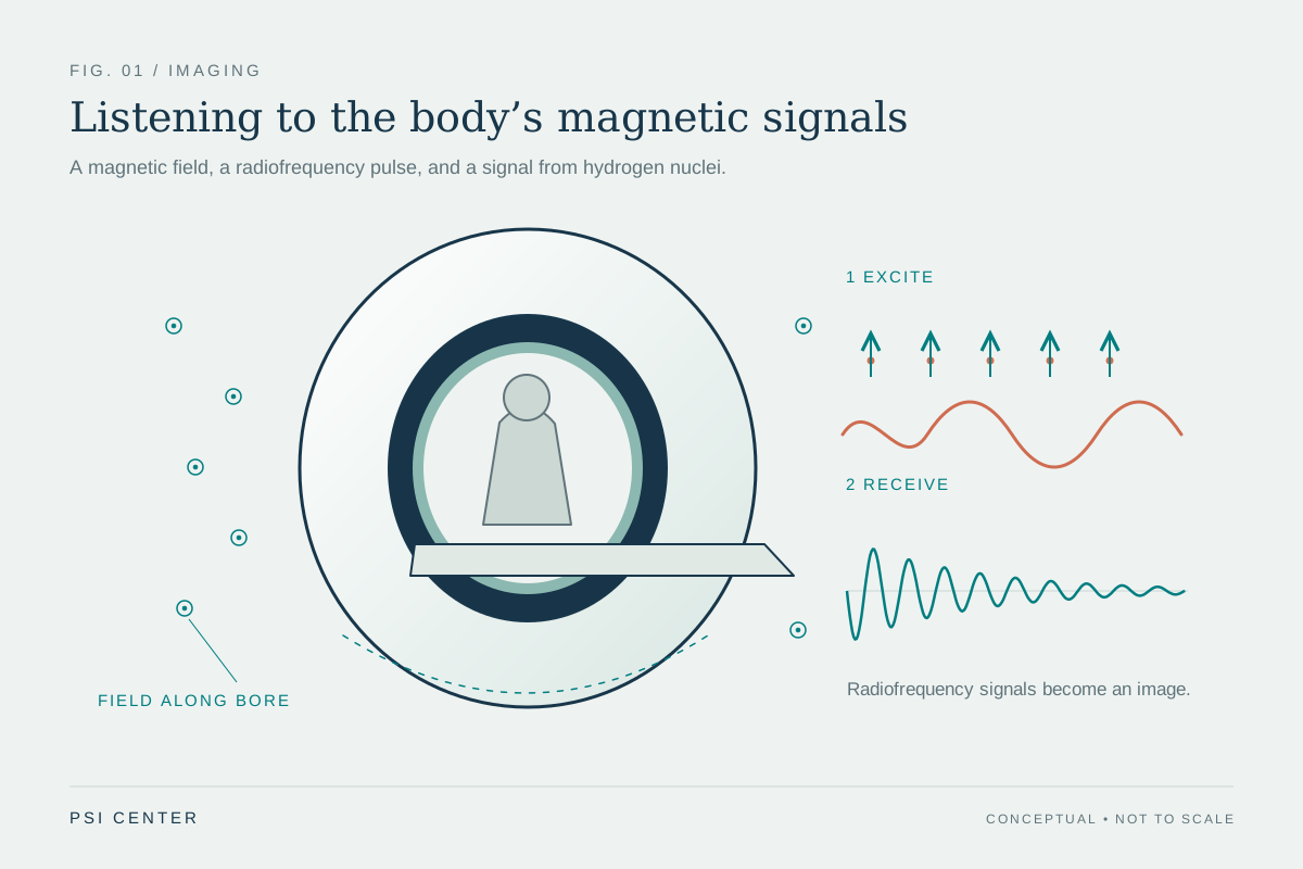
An oscillating radiofrequency magnetic field near resonance can rotate the net magnetization away from its equilibrium direction. In the rotating-frame description, a resonant pulse produces a controllable rotation; the resulting angle depends on the applied RF field and its duration. A nominal 90-degree excitation places equilibrium magnetization in the transverse plane under the ideal model. It does not mean that every proton has become a perfectly aligned little compass, or that the pulse has created a new supply of hydrogen. [8]
After excitation, the transverse magnetization precesses and produces an oscillating electrical signal. The receiver compares that signal with a reference oscillation, preserving both amplitude and phase. This phase information will become essential for locating signal in space. [12]
3. T1, T2, and T2* describe different changes
T1 characterizes the approach of longitudinal magnetization toward thermal equilibrium. Energy exchange between the spin system and its surroundings is involved; fluctuating molecular interactions help determine how efficiently that exchange occurs. T2 characterizes decay of coherent transverse magnetization. The two processes occur together, but they do not describe the same quantity. Their values also depend on material and measurement conditions. [5]
In a simple single-component model, longitudinal recovery after complete saturation follows Mz(t) = M₀[1 − exp(−t/T1)], while transverse decay follows Mxy(t) = Mxy(0)exp(−t/T2). These are model equations, not guarantees that every voxel contains one exponential. A voxel may mix several environments with different relaxation behavior. [7]
Additional differences in local precession frequency cause further transverse dephasing. A freely observed signal therefore often decays with the shorter effective time T2*. Some of that dephasing can be reversible: an ideal spin-echo refocusing pulse makes stationary frequency offsets rephase. It cannot restore coherence already lost through the underlying T2 processes. Hahn’s original echo experiments demonstrated that a signal disappearing through dephasing need not represent irreversible loss of all recoverable information. [6]
A gradient echo reverses an applied gradient’s phase accumulation. It generally retains sensitivity to static field inhomogeneity that an ideal spin echo can refocus. That distinction helps explain why two acquisitions with similar nominal resolution can respond very differently near susceptibility variations. [10]
| Quantity | What changes | Important distinction |
|---|---|---|
| T1 | Longitudinal magnetization recovers toward equilibrium | Recovery is not the same as transverse phase coherence. |
| T2 | Coherent transverse magnetization decays | An ideal refocusing pulse does not reverse this underlying decay. |
| T2* | Observed transverse signal includes extra dephasing | Static frequency differences can contribute reversible dephasing. |
4. Gradients make frequency and phase depend on position
A receiver coil initially hears contributions from an extended volume. To build an image, the experiment needs a reproducible relationship between position and the measured signal. Magnetic-field gradients provide it. To first approximation, the component of field along the main field becomes Bz(r) = B₀ + G·r. Here G describes the spatial slope of that component, in tesla per metre. The x, y, and z gradient labels do not mean that the main field simply points in three different directions. [9]
While a gradient is present, different positions have different resonance frequencies. During a readout gradient, this supplies frequency encoding. A gradient applied earlier can instead leave different positions with different phases after it switches off. The accumulated phase depends on the gradient’s time integral. Repeating an experiment with different gradient areas supplies different spatial encodings; changing only the receiver’s display cannot supply the missing measurements. [12]
Slice selection combines a gradient with an RF pulse that covers a selected frequency band. Because resonance frequency varies with position, that band corresponds approximately to a slab. In an ideal linear-gradient model, slab thickness is Δz ≈ Δf/(γ̄|Gz|), where Δf is the RF bandwidth in hertz. A real pulse has a finite transition region, so a slice is a sensitivity profile rather than an infinitely sharp wall. [11]
These are encoding principles, not operator instructions. Real sequences must coordinate excitation, refocusing, gradient timing, hardware limits, and the signal evolution already underway. The useful abstraction is that a controlled magnetic history writes spatial information into phase.
5. Why the measured signal is a Fourier measurement
Define k(t) = γ̄∫G(t′)dt′. Its units are cycles per metre: multiplying by a position in metres gives cycles, and multiplying again by 2π gives phase in radians. In a simple Cartesian acquisition, successive gradient histories choose successive values of this spatial-frequency coordinate. This is why gradient area, rather than gradient amplitude alone, determines the accumulated spatial encoding. [9]
For a stationary object and an idealized encoding model, the received signal can be written s(k) = ∫m(r)exp(−i2πk·r)dr. The effective complex object m includes the magnetization available to the sequence and, for one receive channel, the coil’s spatial sensitivity. The exponential describes a spatial pattern of phase. The measured complex number is the sum of all contributions after weighting them by that pattern. [12]
This equation is a Fourier transform. Its inverse combines enough spatial-frequency measurements to estimate the object. A k-space sample is therefore not a miniature photograph of one corresponding anatomical point. Every contributing location can affect it. Likewise, reconstructing one image voxel generally combines many measured samples.
The equation also states its own limitations. It treats the effective object as consistent across the measurements being combined. Relaxation during acquisition, off-resonance, motion, flow, and imperfect gradient behavior can violate that simplification. Reconstruction may then need a richer encoding model. A successful Fourier calculation is not evidence that every physical assumption behind it was satisfied.
6. K-space is a map of spatial variation
Small |k| describes slowly varying spatial patterns; large |k| describes more rapid variation. Smooth, broad structures tend to have substantial low-frequency content, whereas sharply defined boundaries require higher spatial frequencies. But an edge is not stored in one outer sample, nor is tissue contrast confined to a central compartment. The final intensity pattern comes from adding all the sampled components with their measured phases. [13]
A simple deduction makes the importance of phase concrete. Suppose an object moves rigidly by a displacement a, without changing shape. In the Fourier integral, substituting r = u + a introduces a factor exp(−i2πk·a). The k-space magnitude can remain unchanged while its phase acquires a ramp. Position has changed even though the magnitude spectrum has not. Keeping amplitude while discarding phase therefore loses spatial information.
The same reasoning explains why inconsistent motion during acquisition is troublesome. If different samples describe different positions, there may be no single stationary object whose Fourier transform matches the entire collection. Ghosts, blur, or other inconsistencies can appear even when the planned sampling grid is complete. More samples do not automatically repair a mismatch between the object’s motion and the reconstruction model.
Calling k-space “raw data” is useful only if we remember that it is already encoded, electronically detected, and calibrated data. Coils, timing, field conditions, and reconstruction conventions influence its interpretation. The image is a physically constrained estimate assembled from measurements, rather than a direct optical view.
7. Worked example: field of view and resolution are different
Consider a stationary one-dimensional phantom, uniformly sampled along one Cartesian k-space direction. For this ideal discrete-Fourier model, field of view is FOV = 1/Δk, where Δk is the spacing between samples. Nominal image spacing is Δx = FOV/N for N acquired samples. The total acquired k-space span controls the scale of resolvable detail; the spacing between samples controls the repetition distance of the reconstructed object. [13]
Choose a 0.240 m field of view and 128 samples. Then Δk = 1/0.240 = 4.1667 cycles/m, and Δx = 0.240/128 = 0.001875 m, or 1.875 mm. The sampled span is approximately NΔk = 533.3 cycles/m. Exact endpoint conventions differ by one sample; that small bookkeeping distinction does not change the sampling argument.
Now retain every other sample while reaching approximately the same outer k-space extent. There are 64 samples separated by 8.3333 cycles/m. Their effective field of view is 0.120 m, while nominal spacing remains 1.875 mm. The penalty is spatial ambiguity: contributions separated by 0.120 m have indistinguishable phase progressions on this coarser grid. Signal outside the smaller field can fold into it. This is aliasing, rather than a simple doubling of pixel size.
These numbers are an independently calculated phantom example, assuming no additional coil encoding or reconstruction prior. They separate two operations often confused in discussion: extending the acquired frequency range can support finer detail; sampling that range more densely can support a larger unambiguous field of view. Neither follows merely from exporting a larger image.
8. Reconstruction cannot manufacture unmeasured detail
With a complete uniform Cartesian grid and the ideal model above, a discrete inverse Fourier transform provides a natural reconstruction. Other trajectories need additional operations, such as interpolation onto a grid or solving the encoding equations directly. The choice should reflect where measurements were made and how their signals evolved. [16]
Even complete coverage of a finite grid does not measure arbitrarily high spatial frequencies. Truncating the spectrum gives the reconstruction a finite point-spread function: a mathematical point spreads into a pattern instead of remaining infinitesimal. An abrupt frequency cutoff produces oscillatory ringing near sharp boundaries. Applying a smoother frequency window can reduce ringing while broadening that response and sacrificing some apparent sharpness. [14]
Zero filling offers a useful distinction. If the 128-sample phantom dataset is padded with zeros and displayed with 256 pixels across 240 mm, the displayed spacing becomes 0.9375 mm. No additional high-frequency measurements have appeared. The display samples an interpolated reconstruction more finely; it does not establish that two objects 0.9375 mm apart can be independently resolved.
Artifacts also have different causes. Coarse sampling can cause aliasing; finite coverage can cause ringing; an inaccurate field model can distort position; inconsistent motion can produce ghosts. A clean-looking image may still have limited resolution, and a visibly imperfect image may retain useful information. Evaluating reconstruction requires attention to spatial response, noise, and fidelity to the measurements, rather than smoothness alone.
9. Image contrast depends on the experiment
MRI can reveal soft-tissue differences because signal depends on properties such as mobile proton content and relaxation behavior, together with the acquisition used to interrogate them. The same anatomy can therefore look substantially different in different sequences. That flexibility is a central strength of MRI, but it makes brightness a conditional observation. [1]
A common simplified spin-echo expression is S ∝ ρ[1 − exp(−TR/T1)]exp(−TE/T2). Here ρ represents effective MR-visible proton density, TR is the repetition interval, and TE is the echo time. This approximation assumes ideal pulses, a simple tissue model, negligible flow and exchange, and an echo-formation interval short relative to TR. Coil sensitivity and other scale factors are omitted. It explains weighting, rather than fully predicting every real sequence. [16]
The expression shows why a brighter voxel has several possible explanations. It may contain more contributing signal, recover longitudinal magnetization differently, lose transverse coherence differently, or experience a different receive sensitivity. If TR is very long compared with the relevant T1 values, the recovery factors approach one and T1 differences contribute less. If TE is very short compared with the relevant T2 values, less T2 decay has occurred. These limiting cases are mathematical observations, not suggested examination settings.
A T1-weighted image is not automatically a numerical T1 map. Mapping requires multiple appropriately varied measurements, fitting, and a model whose assumptions are examined. Nor does an unusual intensity identify a disease by itself. Diagnosis combines the pattern across images with anatomy, clinical context, and other evidence.
10. Worked example: a smaller voxel collects less signal
Signal-to-noise ratio compares a signal estimate with the scale of its fluctuations. Receive coils detect thermal noise as well as signal, and noise can arise substantially from the sample itself. Coil geometry, coupling, receiver bandwidth, and field conditions matter; there is no universal rule converting field strength alone into image quality. [17]
For a deliberately controlled phantom example, keep in-plane sampling, readout bandwidth, coil, field, sequence contrast, and acquisition timing fixed. Change only an ideal uniform slice thickness from 4 mm to 2 mm. With 1.5 mm × 1.5 mm in-plane dimensions, voxel volume falls from 9 mm³ to 4.5 mm³. Assume uniform material, perfect slice profiles, and unchanged receiver noise. The collected signal then halves, so an initial SNR of 30 becomes approximately 15. The smaller voxel reduces mixing across the slice but supplies less signal. [15]
Averaging four independent repetitions would raise that SNR by √4 = 2, returning it to approximately 30 while requiring four times the repeated measurement duration. This follows because coherent signal adds directly while independent random-noise variances add. Motion, drift, and systematic errors do not obey this simple noise-reduction promise. The example is a model comparison, not guidance for changing a clinical examination.
Time also pays for encoding. In a basic conventional two-dimensional sequence acquiring one phase-encoding line per repetition, duration is approximately TR × number of phase encodes × number of averages. Echo trains, parallel imaging, preparation pulses, and other sequence details change that accounting. Improving resolution can simultaneously reduce signal per voxel and demand additional encoding; the consequences depend on what else is held fixed. [11]
11. Faster imaging trades on additional information or assumptions
Parallel imaging adds spatial information from multiple receiver coils. Each coil has a different sensitivity pattern, so its signal weights locations differently. SENSE, introduced by Pruessmann and colleagues, uses those sensitivity differences to reconstruct images with fewer conventional gradient-encoded measurements. This supplements Fourier encoding rather than simply accepting a folded image. [18]
An inverse-problem consequence is that separation becomes unreliable when the available sensitivity patterns distinguish locations poorly. Measurement noise and sensitivity-model errors then matter strongly. “More coils” is not itself a guarantee that every acceleration factor preserves the same information everywhere. This is a mathematical limitation of recovering several unknown contributions from imperfectly independent measurements.
Compressed sensing uses another kind of structure. Lustig and colleagues’ Sparse MRI work combined incoherent undersampling, sparsity in a suitable transform, and nonlinear reconstruction. The reconstruction seeks an image compatible with the acquired measurements while favoring a compact representation. It does not assert that every possible object can be recovered from arbitrarily few measurements. [19]
Data fidelity constrains measured samples; assumptions help choose among possibilities at unmeasured locations. If those assumptions fit poorly, some features may be smoothed, biased, or confused with artifacts. The relevant question is therefore task-specific: does a faster acquisition preserve the features and uncertainty that matter for its intended use? A pleasing reconstruction is useful evidence only when evaluated alongside measurements, validation, and the limits of its model.
12. The physics also defines the safety boundaries
MRI uses nonionizing radiofrequency energy rather than the ionizing X-rays used in CT. That distinction does not remove physical hazards. A strong static field can exert forces on magnetic objects; rapidly switched gradients can produce loud sound and peripheral nerve stimulation; RF energy can heat tissue and contribute to burns. Each hazard comes from a different part of the same apparatus used to create and encode signal. [2]
Device labeling also requires precision. MR Conditional means safety has been demonstrated under specified conditions, not that an implant or accessory is compatible with every scanner and sequence. Device identity, field conditions, configuration, and the manufacturer’s restrictions matter. Safety screening and examination planning belong within the clinical MRI workflow; the numerical models in this article cannot establish a person’s eligibility or a device’s compatibility. [2]
The larger lesson is that an MRI image carries a chain of dependencies: an equilibrium spin population, an excitation history, relaxation, spatial encoding, electrical detection, and an inverse calculation. Knowing that chain makes both the achievements and the limits easier to judge. A voxel is a finite estimate with a particular spatial response, contrast, and noise level. Its meaning comes from understanding the experiment that produced it, then interpreting it in the appropriate diagnostic context.
Explore the physics: an explanatory diagram
Sources & further reading
- Magnetic Resonance Imaging NIBIB
- MRI Benefits and Risks FDA
- CODATA value: proton gyromagnetic ratio in MHz/T National Institute of Standards and Technology
- Nuclear Induction — Felix Bloch (1946) Physical Review / American Physical Society
- Relaxation Effects in Nuclear Magnetic Resonance Absorption — Bloembergen, Purcell, and Pound (1948) Physical Review / American Physical Society
- Spin Echoes — Erwin L. Hahn (1950) Physical Review / American Physical Society
- Notes on NMR Physics — Douglas C. Noll University of Michigan, BME 483
- The Rotating Frame, RF Pulses and the Bloch Equations — David Cory MIT OpenCourseWare, course 22.920
- Magnetization Gradients, k-space and Molecular Diffusion — David Cory MIT OpenCourseWare, course 22.920
- Gradient and Spin Echoes — David Cory MIT OpenCourseWare, course 22.920
- 2-D Imaging and Slice Selection — David Cory MIT OpenCourseWare, course 22.920
- Notes on MRI, Part II — Douglas C. Noll University of Michigan, BME 483
- Notes on MRI, Part III — Douglas C. Noll University of Michigan, BME 483
- Notes on 1D and 2D Fourier Transforms — Douglas C. Noll University of Michigan, BME 483
- Imaging Notes, Part IV — Douglas C. Noll University of Michigan, BME 483
- RAD229 MRI Signals: course notes — Brian Hargreaves (2017) Stanford University
- The intrinsic signal-to-noise ratio in NMR imaging — Edelstein and colleagues (1986) Magnetic Resonance in Medicine / Wiley
- SENSE: sensitivity encoding for fast MRI — Pruessmann and colleagues (1999) Magnetic Resonance in Medicine; abstract via PubMed
- Sparse MRI: The application of compressed sensing for rapid MR imaging — Lustig, Donoho, and Pauly (2007) Magnetic Resonance in Medicine; abstract via PubMed
Sources checked: 30 October 2026. The calculations illustrate physical models; they are not clinical settings.
Prepared for the independent PSI Center reading library. About edition dates and source checking.
This explainer describes scientific principles. It does not assess individual treatment choices.